Fitting pressure-volume curves

fit_PV_curve(
  data,
  varnames = list(psi = "psi", mass = "mass", leaf_mass = "leaf_mass", bag_mass =
    "bag_mass", leaf_area = "leaf_area"),
  title = NULL
)

Arguments

data: Dataframe
varnames: Variable names. varnames = list(psi = "psi", mass = "mass", leaf_mass = "leaf_mass", bag_mass = "bag_mass", leaf_area = "leaf_area") where psi is leaf water potential in MPa, mass is the weighed mass of the bag and leaf in g, leaf_mass is the mass of the leaf in g, bag_mass is the mass of the bag in g, and leaf_area is the area of the leaf in cm2.
title: Graph title

Value

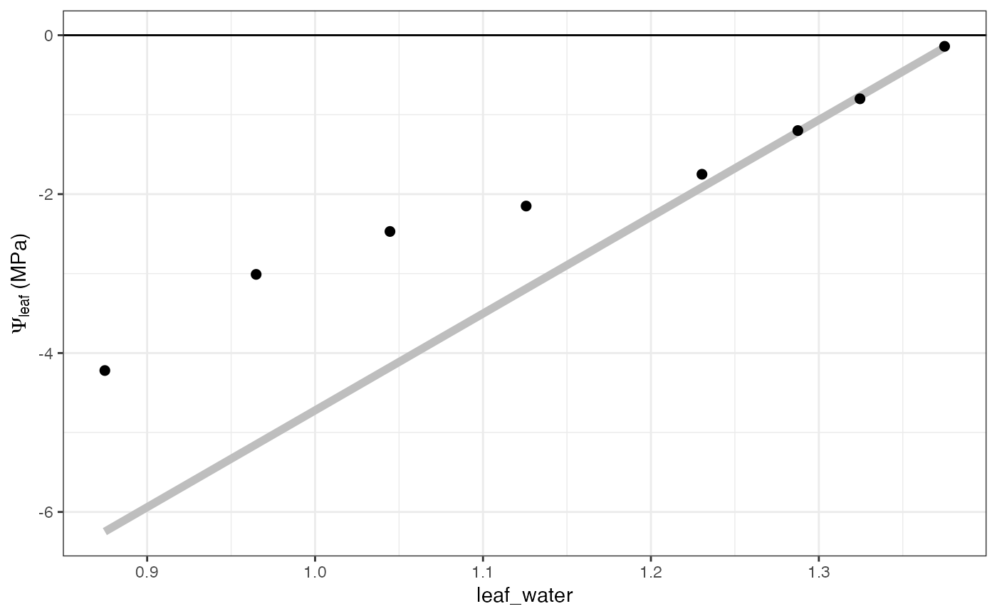
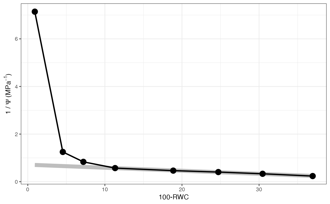
fit_PV_curve fits pressure-volume curve data to determine: SWC: saturated water content per leaf mass (g H2O g leaf dry mass ^ -1), PI_o: osmotic potential at full turgor (MPa), psi_TLP: leaf water potential at turgor loss point (TLP) (MPa), RWC_TLP: relative water content at TLP (%), eps: modulus of elasticity at full turgor (MPa), C_FT: relative capacitance at full turgor (MPa ^ -1), C_TLP: relative capacitance at TLP (MPa ^ -1), and C_FTStar: absolute capacitance per leaf area (g m ^ -2 MPa ^ -1). Element 1 of the output list contains the fitted parameters, element 2 contains the water-psi graph, and element 3 contains the 1/psi-100-RWC graph.

References

Koide RT, Robichaux RH, Morse SR, Smith CM. 2000. Plant water status, hydraulic resistance and capacitance. In: Plant Physiological Ecology: Field Methods and Instrumentation (eds RW Pearcy, JR Ehleringer, HA Mooney, PW Rundel), pp. 161-183. Kluwer, Dordrecht, the Netherlands

Sack L, Cowan PD, Jaikumar N, Holbrook NM. 2003. The 'hydrology' of leaves: co-ordination of structure and function in temperate woody species. Plant, Cell and Environment, 26, 1343-1356

Tyree MT, Hammel HT. 1972. Measurement of turgor pressure and water relations of plants by pressure bomb technique. Journal of Experimental Botany, 23, 267

Examples

# \donttest{
# Read in data
data <- read.csv(system.file("extdata", "PV_curve.csv",
  package = "photosynthesis"
))

# Fit one PV curve
fit <- fit_PV_curve(data[data$ID == "L2", ],
  varnames = list(
    psi = "psi",
    mass = "mass",
    leaf_mass = "leaf_mass",
    bag_mass = "bag_mass",
    leaf_area = "leaf_area"
  )
)

# See fitted parameters
fit[[1]]
#>        SWC      PI_o psi_TLP  RWC_TLP      eps       C_FT      C_TLP  C_FTStar
#> 1 2.438935 -1.399302   -1.75 88.67684 12.20175 0.06456207 0.09923338 0.5161476

# Plot water mass graph
fit[[2]]


# Plot PV Curve
fit[[3]]


# Fit all PV curves in a file
fits <- fit_many(data,
  group = "ID",
  funct = fit_PV_curve,
  varnames = list(
    psi = "psi",
    mass = "mass",
    leaf_mass = "leaf_mass",
    bag_mass = "bag_mass",
    leaf_area = "leaf_area"
  )
)
#> 
  |                                                                            
  |                                                                      |   0%
  |                                                                            
  |=======================                                               |  33%
  |                                                                            
  |===============================================                       |  67%
  |                                                                            
  |======================================================================| 100%

# See parameters
fits[[1]][[1]]
#>        SWC      PI_o psi_TLP  RWC_TLP      eps       C_FT      C_TLP  C_FTStar
#> 1 2.438935 -1.399302   -1.75 88.67684 12.20175 0.06456207 0.09923338 0.5161476

# See water mass - water potential graph
fits[[1]][[2]]


# See PV curve
fits[[1]][[3]]


# Compile parameter outputs
pars <- compile_data(
  data = fits,
  output_type = "dataframe",
  list_element = 1
)

# Compile the water mass - water potential graphs
graphs1 <- compile_data(
  data = fits,
  output_type = "list",
  list_element = 2
)

# Compile the PV graphs
graphs2 <- compile_data(
  data = fits,
  output_type = "list",
  list_element = 3
)
# }