![[Deprecated]](figures/lifecycle-deprecated.svg)
Please use fit_aq_response2().
Usage
fit_aq_response(
  data,
  varnames = list(A_net = "A_net", PPFD = "PPFD"),
  usealpha_Q = FALSE,
  alpha_Q = 0.84,
  title = NULL
)
Arguments
- data
Dataframe containing CO2 assimilation light response
- varnames
Variable names where varnames = list(A_net = "A_net", PPFD = "PPFD"). A_net is net CO2 assimilation in umol m-2 s-1, PPFD is incident irradiance. PPFD can be corrected for light absorbance by using useapha_Q and setting alpha_Q.
- usealpha_Q
Correct light intensity for absorbance? Default is FALSE.
- alpha_Q
Absorbance of incident light. Default value is 0.84.
- title
Title for graph
Value
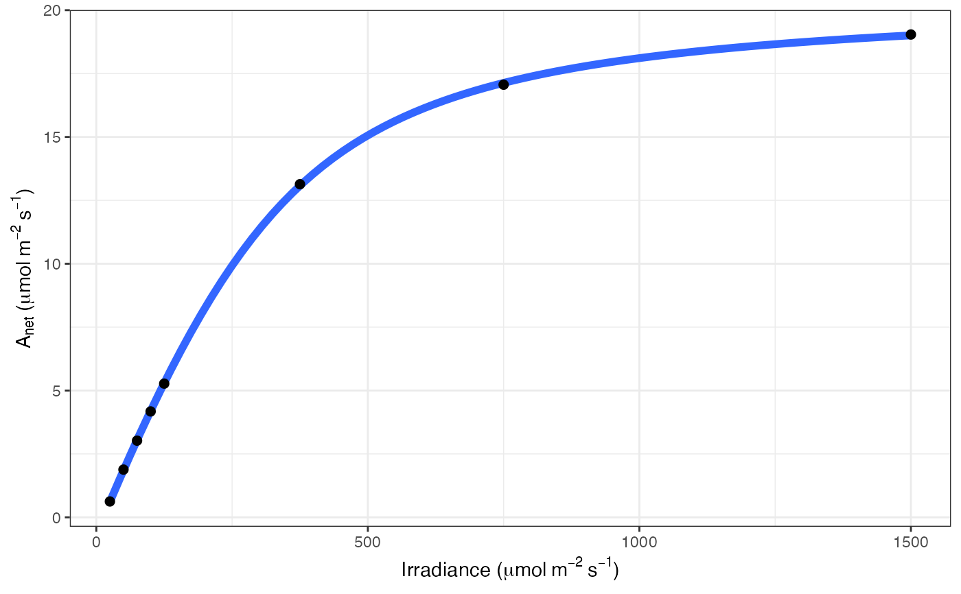
fit_aq_response fits the light response of net CO2 assimilation. Output is a dataframe containing light saturated net CO2 assimilation, quantum yield of CO2 assimilation (phi_J), curvature of the light response (theta_J), respiration (Rd), light compensation point (LCP), and residual sum of squares (resid_SS). Note that Rd fitted in this way is essentially the same as the Kok method, and represents a respiration value in the light that may not be accurate. Rd output should thus be interpreted more as a residual parameter to ensure an accurate fit of the light response parameters. Model originally from Marshall & Biscoe 1980.
References
Marshall B, Biscoe P. 1980. A model for C3 leaves describing the dependence of net photosynthesis on irradiance. J Ex Bot 31:29-39
Examples
# \donttest{
# Read in your data
# Note that this data is coming from data supplied by the package
# hence the complicated argument in read.csv()
# This dataset is a CO2 by light response curve for a single sunflower
data = read.csv(system.file("extdata", "A_Ci_Q_data_1.csv",
package = "photosynthesis"
))
# Fit many AQ curves
# Set your grouping variable
# Here we are grouping by CO2_s and individual
data$C_s = (round(data$CO2_s, digits = 0))
# For this example we need to round sequentially due to CO2_s setpoints
data$C_s = as.factor(round(data$C_s, digits = -1))
# To fit one AQ curve
fit = fit_aq_response(data[data$C_s == 600, ],
varnames = list(
A_net = "A",
PPFD = "Qin"
)
)
#> Warning: `fit_aq_response()` was deprecated in photosynthesis 2.1.1.
#> ℹ Please use the `.photo_fun` argument of `fit_photosynthesis()` instead.
#> Warning: `aq_response()` was deprecated in photosynthesis 2.1.1.
#> ℹ Please use `marshall_biscoe_1980()` instead.
#> ℹ The deprecated feature was likely used in the photosynthesis package.
#> Please report the issue at <https://github.com/cdmuir/photosynthesis/issues>.
# Print model summary
summary(fit[[1]])
#>
#> Formula: A_net ~ aq_response(k_sat, phi_J, Q_abs = data$Q_abs, theta_J) -
#> Rd
#>
#> Parameters:
#> Estimate Std. Error t value Pr(>|t|)
#> k_sat 21.167200 0.158332 133.69 1.88e-08 ***
#> phi_J.Q_abs 0.051907 0.001055 49.18 1.02e-06 ***
#> theta_J 0.775484 0.014920 51.98 8.20e-07 ***
#> Rd.(Intercept) 0.668495 0.065235 10.25 0.000511 ***
#> ---
#> Signif. codes: 0 ‘***’ 0.001 ‘**’ 0.01 ‘*’ 0.05 ‘.’ 0.1 ‘ ’ 1
#>
#> Residual standard error: 0.05535 on 4 degrees of freedom
#>
#> Number of iterations to convergence: 5
#> Achieved convergence tolerance: 1.49e-08
#>
# Print fitted parameters
fit[[2]]
#> A_sat phi_J theta_J Rd LCP resid_SSs
#> k_sat 21.1672 0.05190746 0.7754836 0.6684953 12.97289 0.01225491
# Print graph
fit[[3]]
 # Fit many curves
fits = fit_many(
data = data,
varnames = list(
A_net = "A",
PPFD = "Qin",
group = "C_s"
),
funct = fit_aq_response,
group = "C_s"
)
#>
|
| | 0%
|
|======== | 11%
|
|================ | 22%
|
|======================= | 33%
|
|=============================== | 44%
|
|======================================= | 56%
|
|=============================================== | 67%
|
|====================================================== | 78%
|
|============================================================== | 89%
|
|======================================================================| 100%
# Look at model summary for a given fit
# First set of double parentheses selects an individual group value
# Second set selects an element of the sublist
summary(fits[[3]][[1]])
#>
#> Formula: A_net ~ aq_response(k_sat, phi_J, Q_abs = data$Q_abs, theta_J) -
#> Rd
#>
#> Parameters:
#> Estimate Std. Error t value Pr(>|t|)
#> k_sat 7.347423 0.141931 51.768 8.33e-07 ***
#> phi_J.Q_abs 0.027192 0.001511 17.994 5.61e-05 ***
#> theta_J 0.837778 0.030608 27.371 1.06e-05 ***
#> Rd.(Intercept) 0.615283 0.086994 7.073 0.00211 **
#> ---
#> Signif. codes: 0 ‘***’ 0.001 ‘**’ 0.01 ‘*’ 0.05 ‘.’ 0.1 ‘ ’ 1
#>
#> Residual standard error: 0.06799 on 4 degrees of freedom
#>
#> Number of iterations to convergence: 4
#> Achieved convergence tolerance: 1.49e-08
#>
# Print the parameters
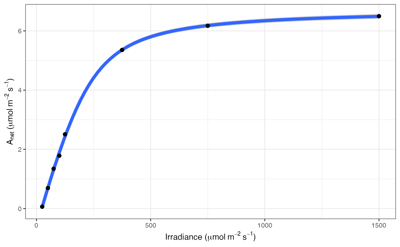
fits[[3]][[2]]
#> A_sat phi_J theta_J Rd LCP resid_SSs
#> k_sat 7.347423 0.02719153 0.8377781 0.6152826 22.96322 0.01849038
# Print the graph
fits[[3]][[3]]
# Fit many curves
fits = fit_many(
data = data,
varnames = list(
A_net = "A",
PPFD = "Qin",
group = "C_s"
),
funct = fit_aq_response,
group = "C_s"
)
#>
|
| | 0%
|
|======== | 11%
|
|================ | 22%
|
|======================= | 33%
|
|=============================== | 44%
|
|======================================= | 56%
|
|=============================================== | 67%
|
|====================================================== | 78%
|
|============================================================== | 89%
|
|======================================================================| 100%
# Look at model summary for a given fit
# First set of double parentheses selects an individual group value
# Second set selects an element of the sublist
summary(fits[[3]][[1]])
#>
#> Formula: A_net ~ aq_response(k_sat, phi_J, Q_abs = data$Q_abs, theta_J) -
#> Rd
#>
#> Parameters:
#> Estimate Std. Error t value Pr(>|t|)
#> k_sat 7.347423 0.141931 51.768 8.33e-07 ***
#> phi_J.Q_abs 0.027192 0.001511 17.994 5.61e-05 ***
#> theta_J 0.837778 0.030608 27.371 1.06e-05 ***
#> Rd.(Intercept) 0.615283 0.086994 7.073 0.00211 **
#> ---
#> Signif. codes: 0 ‘***’ 0.001 ‘**’ 0.01 ‘*’ 0.05 ‘.’ 0.1 ‘ ’ 1
#>
#> Residual standard error: 0.06799 on 4 degrees of freedom
#>
#> Number of iterations to convergence: 4
#> Achieved convergence tolerance: 1.49e-08
#>
# Print the parameters
fits[[3]][[2]]
#> A_sat phi_J theta_J Rd LCP resid_SSs
#> k_sat 7.347423 0.02719153 0.8377781 0.6152826 22.96322 0.01849038
# Print the graph
fits[[3]][[3]]
 # Compile graphs into a list for plotting
fits_graphs = compile_data(fits,
list_element = 3
)
# Compile parameters into dataframe for analysis
fits_pars = compile_data(fits,
output_type = "dataframe",
list_element = 2
)
# }
# Compile graphs into a list for plotting
fits_graphs = compile_data(fits,
list_element = 3
)
# Compile parameters into dataframe for analysis
fits_pars = compile_data(fits,
output_type = "dataframe",
list_element = 2
)
# }