Fitting hydraulic vulnerability curves
Value
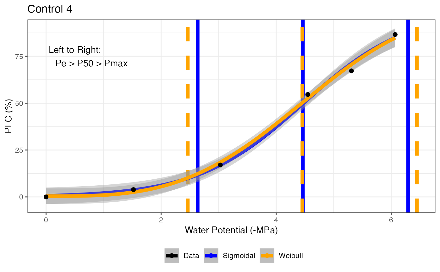
fit_hydra_vuln_curve fits a sigmoidal function (Pammenter & Van der Willigen, 1998) linearized according to Ogle et al. (2009). Output is a list containing the sigmoidal model in element 1 and Weibull model in element 4, the fit parameters with 95% confidence interval for both models are in element 2, and hydraulic parameters in element 3 (including P25, P50, P88, P95, S50, Pe, Pmax, DSI). Px (25 to 95): water potential at which x% of conductivity is lost. S50: slope at 50% loss of conductivity. Pe: air entry point. Pmax: hydraulic failure threshold. DSI: drought stress interval. Element 5 is a graph showing the fit, P50, Pe, and Pmax.
References
Ogle K, Barber JJ, Willson C, Thompson B. 2009. Hierarchical statistical modeling of xylem vulnerability to cavitation. New Phytologist 182:541-554
Pammenter NW, Van der Willigen CV. 1998. A mathematical and statistical analysis of the curves illustrating vulnerability of xylem to cavitation. Tree Physiology 18:589-593
Examples
# \donttest{
# Read in data
data <- read.csv(system.file("extdata", "hydraulic_vulnerability.csv",
package = "photosynthesis"
))
# Fit hydraulic vulnerability curve
fit <- fit_hydra_vuln_curve(data[data$Tree == 4 & data$Plot == "Control", ],
varnames = list(
psi = "P",
PLC = "PLC"
),
title = "Control 4"
)
# Return Sigmoidal model summary
summary(fit[[1]])
#>
#> Call:
#> lm(formula = H_log ~ psi, data = data[data$H_log < Inf, ])
#>
#> Residuals:
#> 38 39 40 41 42
#> -0.01214 0.01361 -0.09323 0.20473 -0.11296
#>
#> Coefficients:
#> Estimate Std. Error t value Pr(>|t|)
#> (Intercept) 4.88183 0.17588 27.76 0.000103 ***
#> psi -1.09305 0.03988 -27.41 0.000107 ***
#> ---
#> Signif. codes: 0 ‘***’ 0.001 ‘**’ 0.01 ‘*’ 0.05 ‘.’ 0.1 ‘ ’ 1
#>
#> Residual standard error: 0.1457 on 3 degrees of freedom
#> Multiple R-squared: 0.996, Adjusted R-squared: 0.9947
#> F-statistic: 751.1 on 1 and 3 DF, p-value: 0.0001066
#>
# Return Weibull model summary
summary(fit[[4]])
#>
#> Formula: K.Kmax ~ exp(-((psi/a)^b))
#>
#> Parameters:
#> Estimate Std. Error t value Pr(>|t|)
#> a 4.99160 0.06222 80.22 1.45e-07 ***
#> b 3.22807 0.22158 14.57 0.000129 ***
#> ---
#> Signif. codes: 0 ‘***’ 0.001 ‘**’ 0.01 ‘*’ 0.05 ‘.’ 0.1 ‘ ’ 1
#>
#> Residual standard error: 0.02427 on 4 degrees of freedom
#>
#> Number of iterations to convergence: 8
#> Achieved convergence tolerance: 1.49e-08
#>
# Return model parameters with 95\% confidence intervals
fit[[2]]
#> Value Parameter Curve
#> b...1 4.466238 b Sigmoidal
#> a...2 -1.093052 a Sigmoidal
#> b...3 3.228068 b Weibull
#> a...4 4.991601 a Weibull
# Return hydraulic parameters
fit[[3]]
#> P25 P50 P88 P95 S50 Pe Pmax DSI
#> 1 3.461151 4.466238 6.289053 7.160017 27.32629 2.636498 6.295978 3.659480
#> 2 3.393285 4.455847 6.300135 7.012168 25.10775 2.464430 6.447264 3.982834
#> Curve
#> 1 Sigmoidal
#> 2 Weibull
# Return graph
fit[[5]]
 # Fit many curves
fits <- fit_many(
data = data,
varnames = list(
psi = "P",
PLC = "PLC"
),
group = "Tree",
funct = fit_hydra_vuln_curve
)
#>
|
| | 0%
|
|============== | 20%
|
|============================ | 40%
|
|========================================== | 60%
|
|======================================================== | 80%
|
|======================================================================| 100%
# To select individuals from the many fits
# Return model summary
summary(fits[[1]][[1]]) # Returns model summary
#>
#> Call:
#> lm(formula = H_log ~ psi, data = data[data$H_log < Inf, ])
#>
#> Residuals:
#> Min 1Q Median 3Q Max
#> -0.6650 -0.4293 0.0984 0.3096 0.8015
#>
#> Coefficients:
#> Estimate Std. Error t value Pr(>|t|)
#> (Intercept) 4.8662 0.4452 10.93 4.35e-06 ***
#> psi -1.0439 0.1010 -10.34 6.61e-06 ***
#> ---
#> Signif. codes: 0 ‘***’ 0.001 ‘**’ 0.01 ‘*’ 0.05 ‘.’ 0.1 ‘ ’ 1
#>
#> Residual standard error: 0.5216 on 8 degrees of freedom
#> Multiple R-squared: 0.9304, Adjusted R-squared: 0.9217
#> F-statistic: 106.9 on 1 and 8 DF, p-value: 6.607e-06
#>
# Return sigmoidal model output
fits[[1]][[2]]
#> Value Parameter Curve
#> b...1 4.661514 b Sigmoidal
#> a...2 -1.043902 a Sigmoidal
#> b...3 3.433237 b Weibull
#> a...4 5.297359 a Weibull
# Return hydraulic parameters
fits[[1]][[3]]
#> P25 P50 P88 P95 S50 Pe Pmax DSI
#> 1 3.609104 4.661514 6.570151 7.482123 26.09754 2.745624 6.577403 3.831778
#> 2 3.685164 4.760983 6.593668 7.292066 24.99209 2.760350 6.761615 4.001265
#> Curve
#> 1 Sigmoidal
#> 2 Weibull
# Return graph
fits[[1]][[5]]
# Fit many curves
fits <- fit_many(
data = data,
varnames = list(
psi = "P",
PLC = "PLC"
),
group = "Tree",
funct = fit_hydra_vuln_curve
)
#>
|
| | 0%
|
|============== | 20%
|
|============================ | 40%
|
|========================================== | 60%
|
|======================================================== | 80%
|
|======================================================================| 100%
# To select individuals from the many fits
# Return model summary
summary(fits[[1]][[1]]) # Returns model summary
#>
#> Call:
#> lm(formula = H_log ~ psi, data = data[data$H_log < Inf, ])
#>
#> Residuals:
#> Min 1Q Median 3Q Max
#> -0.6650 -0.4293 0.0984 0.3096 0.8015
#>
#> Coefficients:
#> Estimate Std. Error t value Pr(>|t|)
#> (Intercept) 4.8662 0.4452 10.93 4.35e-06 ***
#> psi -1.0439 0.1010 -10.34 6.61e-06 ***
#> ---
#> Signif. codes: 0 ‘***’ 0.001 ‘**’ 0.01 ‘*’ 0.05 ‘.’ 0.1 ‘ ’ 1
#>
#> Residual standard error: 0.5216 on 8 degrees of freedom
#> Multiple R-squared: 0.9304, Adjusted R-squared: 0.9217
#> F-statistic: 106.9 on 1 and 8 DF, p-value: 6.607e-06
#>
# Return sigmoidal model output
fits[[1]][[2]]
#> Value Parameter Curve
#> b...1 4.661514 b Sigmoidal
#> a...2 -1.043902 a Sigmoidal
#> b...3 3.433237 b Weibull
#> a...4 5.297359 a Weibull
# Return hydraulic parameters
fits[[1]][[3]]
#> P25 P50 P88 P95 S50 Pe Pmax DSI
#> 1 3.609104 4.661514 6.570151 7.482123 26.09754 2.745624 6.577403 3.831778
#> 2 3.685164 4.760983 6.593668 7.292066 24.99209 2.760350 6.761615 4.001265
#> Curve
#> 1 Sigmoidal
#> 2 Weibull
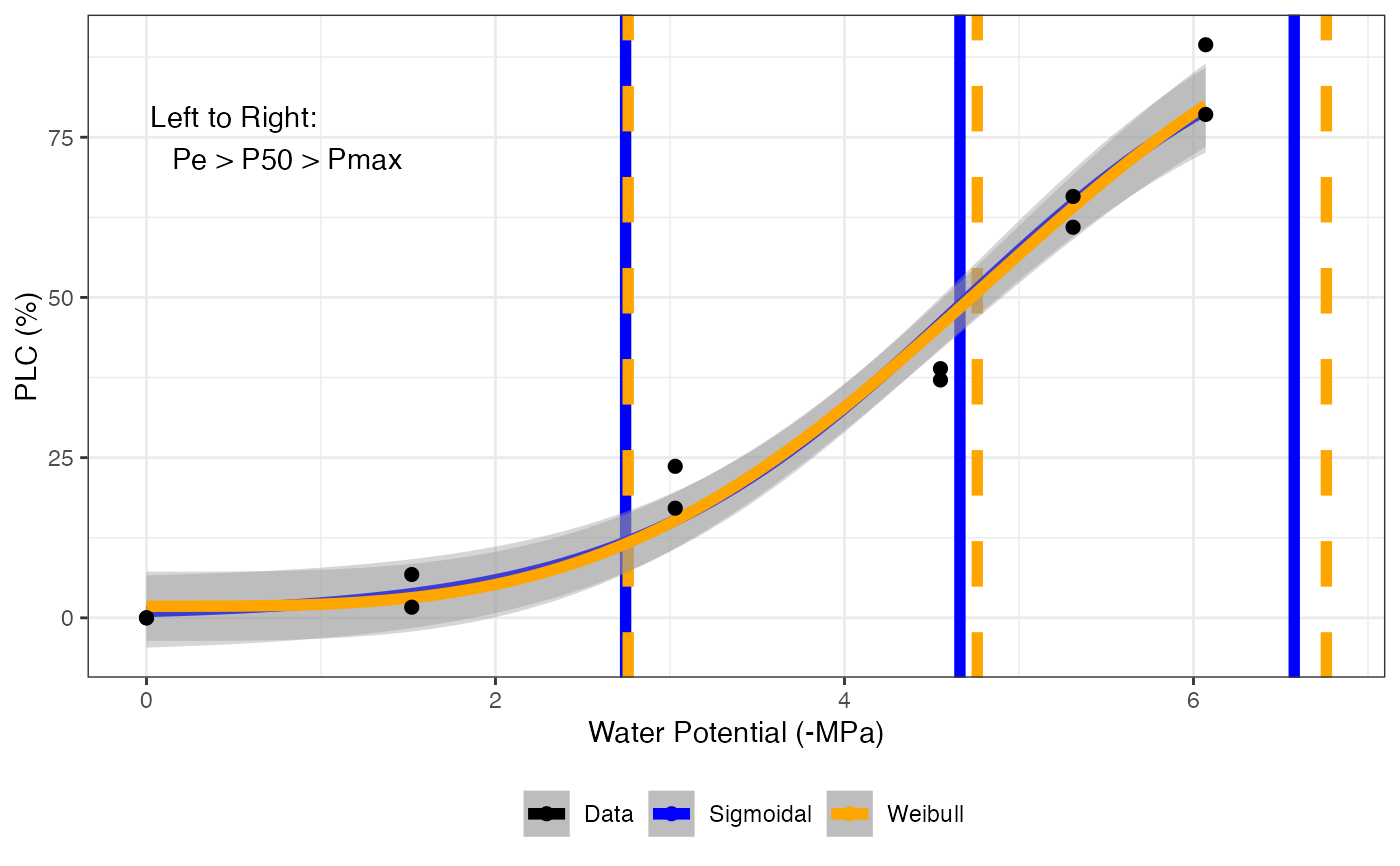
# Return graph
fits[[1]][[5]]
 # Compile parameter outputs
pars <- compile_data(
data = fits,
output_type = "dataframe",
list_element = 3
)
# Compile graphs
graphs <- compile_data(
data = fits,
output_type = "list",
list_element = 5
)
# }
# Compile parameter outputs
pars <- compile_data(
data = fits,
output_type = "dataframe",
list_element = 3
)
# Compile graphs
graphs <- compile_data(
data = fits,
output_type = "list",
list_element = 5
)
# }