Printing graphs to system

print_graphs(
  data,
  path,
  output_type = "jpeg",
  height = 5,
  width = 5,
  res = 600,
  units = "in",
  pdf_filename,
  ...
)

Arguments

data: List of graphs
path: File path for printing our graphs. Use "./" to set to current working directory
output_type: Type of output file, jpeg or pdf
height: Height of jpegs
width: Width of jpegs
res: Resolution of jpegs
units: Units of height and width
pdf_filename: Filename for pdf option
...: Further arguments for jpeg() and pdf()

Value

print_graphs creates graph files in current working directory from a list of graphs

Examples

# \donttest{
# Read in your data
# Note that this data is coming from data supplied by the package
# hence the complicated argument in read.csv()
# This dataset is a CO2 by light response curve for a single sunflower
data <- read.csv(system.file("extdata", "A_Ci_Q_data_1.csv",
  package = "photosynthesis"
))

# Fit many AQ curves
# Set your grouping variable
# Here we are grouping by CO2_s and individual
data$C_s <- (round(data$CO2_s, digits = 0))

# For this example we need to round sequentially due to CO2_s setpoints
data$C_s <- as.factor(round(data$C_s, digits = -1))

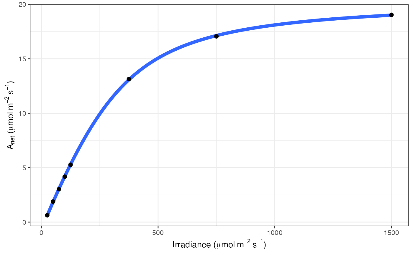
# To fit one AQ curve
fit <- fit_aq_response(data[data$C_s == 600, ],
  varnames = list(
    A_net = "A",
    PPFD = "Qin"
  )
)

# Print model summary
summary(fit[[1]])
#> 
#> Formula: A_net ~ aq_response(k_sat, phi_J, Q_abs = data$Q_abs, theta_J) - 
#>     Rd
#> 
#> Parameters:
#>                 Estimate Std. Error t value Pr(>|t|)    
#> k_sat          21.167200   0.158332  133.69 1.88e-08 ***
#> phi_J.Q_abs     0.051907   0.001055   49.18 1.02e-06 ***
#> theta_J         0.775484   0.014920   51.98 8.20e-07 ***
#> Rd.(Intercept)  0.668495   0.065235   10.25 0.000511 ***
#> ---
#> Signif. codes:  0 ‘***’ 0.001 ‘**’ 0.01 ‘*’ 0.05 ‘.’ 0.1 ‘ ’ 1
#> 
#> Residual standard error: 0.05535 on 4 degrees of freedom
#> 
#> Number of iterations to convergence: 5 
#> Achieved convergence tolerance: 1.49e-08
#> 

# Print fitted parameters
fit[[2]]
#>         A_sat      phi_J   theta_J        Rd      LCP  resid_SSs
#> k_sat 21.1672 0.05190746 0.7754836 0.6684953 12.97289 0.01225491

# Print graph
fit[[3]]


# Fit many curves
fits <- fit_many(
  data = data,
  varnames = list(
    A_net = "A",
    PPFD = "Qin",
    group = "C_s"
  ),
  funct = fit_aq_response,
  group = "C_s"
)
#> 
  |                                                                            
  |                                                                      |   0%
  |                                                                            
  |========                                                              |  11%
  |                                                                            
  |================                                                      |  22%
  |                                                                            
  |=======================                                               |  33%
  |                                                                            
  |===============================                                       |  44%
  |                                                                            
  |=======================================                               |  56%
  |                                                                            
  |===============================================                       |  67%
  |                                                                            
  |======================================================                |  78%
  |                                                                            
  |==============================================================        |  89%
  |                                                                            
  |======================================================================| 100%

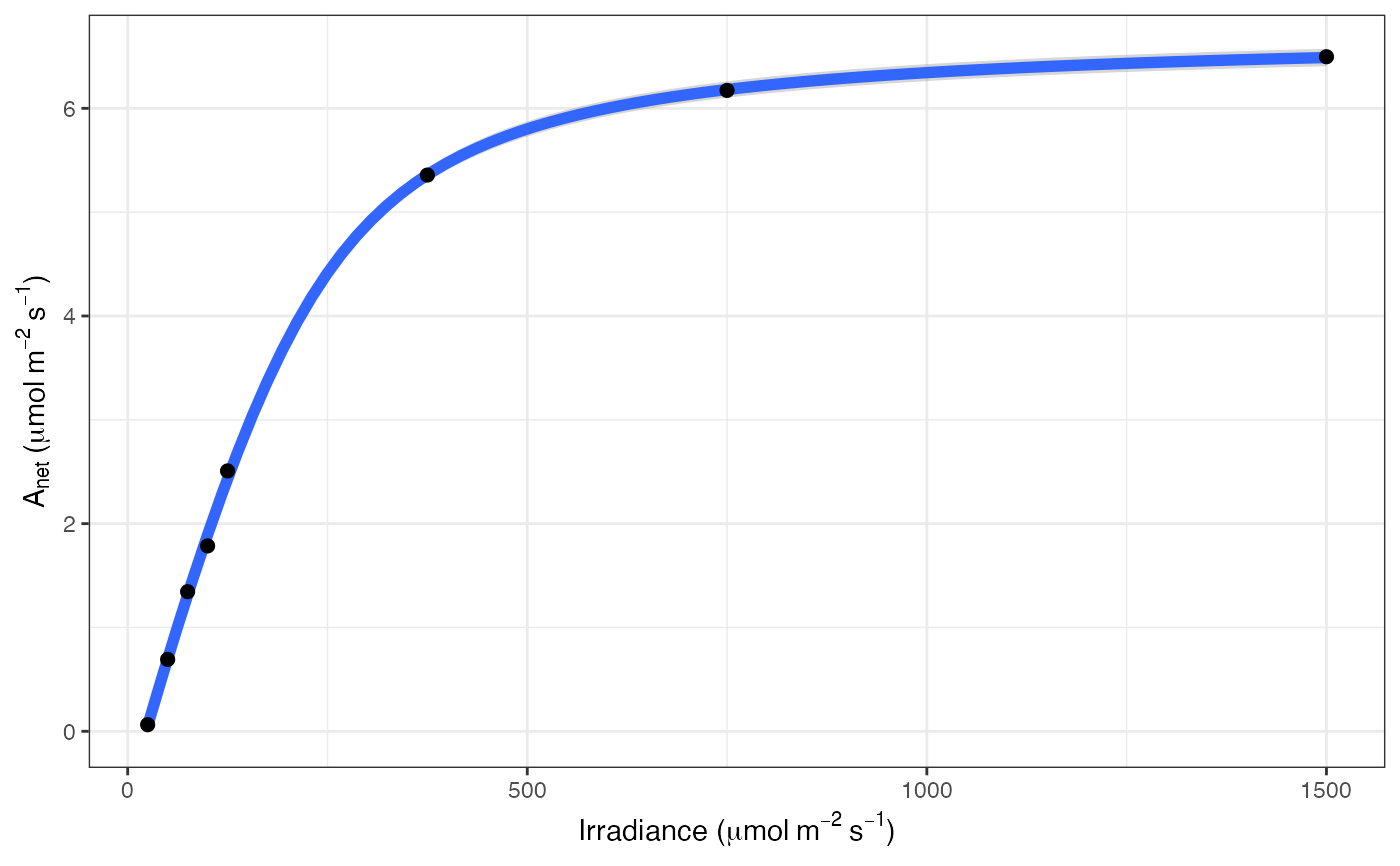
# Look at model summary for a given fit
# First set of double parentheses selects an individual group value
# Second set selects an element of the sublist
summary(fits[[3]][[1]])
#> 
#> Formula: A_net ~ aq_response(k_sat, phi_J, Q_abs = data$Q_abs, theta_J) - 
#>     Rd
#> 
#> Parameters:
#>                Estimate Std. Error t value Pr(>|t|)    
#> k_sat          7.347423   0.141931  51.768 8.33e-07 ***
#> phi_J.Q_abs    0.027192   0.001511  17.994 5.61e-05 ***
#> theta_J        0.837778   0.030608  27.371 1.06e-05 ***
#> Rd.(Intercept) 0.615283   0.086994   7.073  0.00211 ** 
#> ---
#> Signif. codes:  0 ‘***’ 0.001 ‘**’ 0.01 ‘*’ 0.05 ‘.’ 0.1 ‘ ’ 1
#> 
#> Residual standard error: 0.06799 on 4 degrees of freedom
#> 
#> Number of iterations to convergence: 4 
#> Achieved convergence tolerance: 1.49e-08
#> 

# Print the parameters
fits[[3]][[2]]
#>          A_sat      phi_J   theta_J        Rd      LCP  resid_SSs
#> k_sat 7.347423 0.02719153 0.8377781 0.6152826 22.96322 0.01849038

# Print the graph
fits[[3]][[3]]


# Compile graphs into a list for plotting
fits_graphs <- compile_data(fits,
  list_element = 3
)

# Print graphs to pdf
# Uncomment to run
# print_graphs(data = fits_graphs,
#            output_type = "pdf",
#            path = tempdir(),
#            pdf_filename = "mygraphs.pdf")
# }